Rebote de una pelota
(→Manual Ball Bounce) |
(→Rebote manual de la pelotaFile:Example.jpg) |
||
| Line 19: | Line 19: | ||
#The fourth way to simulate a bouncing ball is to create the mathematical equations to do that. Just make several parabolic shots at the rigth place a the right time to simulate a bouncing ball. It would be a little tricky but probably should be the most accurate one. | #The fourth way to simulate a bouncing ball is to create the mathematical equations to do that. Just make several parabolic shots at the rigth place a the right time to simulate a bouncing ball. It would be a little tricky but probably should be the most accurate one. | ||
| − | == Rebote manual de la pelota[[File:Example.jpg]] | + | == Rebote manual de la pelota == |
| + | |||
| + | [[File:Example.jpg]] | ||
La regla para hacer el rebote manual es dibujar en un papel el rebote deseado. Después marcar la línea horizontal con intervalos regulares y hacerlos coincidir en la intersección de la curva en vertical. Véase la imagen: | La regla para hacer el rebote manual es dibujar en un papel el rebote deseado. Después marcar la línea horizontal con intervalos regulares y hacerlos coincidir en la intersección de la curva en vertical. Véase la imagen: | ||
Revision as of 05:27, 13 November 2011
|
Warning! This page contains outdated information. The release of Synfig Studio 0.64.0 introduced new terminology and this translated page needs to be updated according to original English text. You can help updating this page - see instructions here. Thank you! |
Esta página se está traduciendo. Por favor, ten paciencia.
This is a tutorial to explain how to create a bounce tutorial. The main target of the tutorial covers the ball movement. It is known that cartoon like balls have also a very deformed poses meanwhile thery are travelling and especially when it hits the ground. This could be covered in a second stage.
Contents
Diferentes aproximaciones para el mismo resultado
Con Synfig hay cuatro maneras de crear una pelota rebotando usando las posibilidades técnicas de este programa.
- En la primera se hace el rebote de la pelota manualmente. Eso implicaría crear muchos puntos de interepolación y ajustarlos para concordar con un movimiento parabólico (en tiempo y trayectoria).
- La segunda manera es usar parámetros de interpolación de los puntos de interpolación (puntos verdes) cuando están colocados en la interpolación TCB. Esto reduciría drásticamente la cifra de interpolaciones y también hace que el tiempo de los rebotes sea más fácil.
- Para la tercera forma se hace uso del enlace con la línea Béizer. Si se dibuja el camino del rebote de la pelota usando una línea Béizer es fácil hacer siga el camino incluso variando la velocidad.
- The fourth way to simulate a bouncing ball is to create the mathematical equations to do that. Just make several parabolic shots at the rigth place a the right time to simulate a bouncing ball. It would be a little tricky but probably should be the most accurate one.
Rebote manual de la pelota
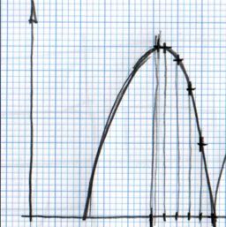
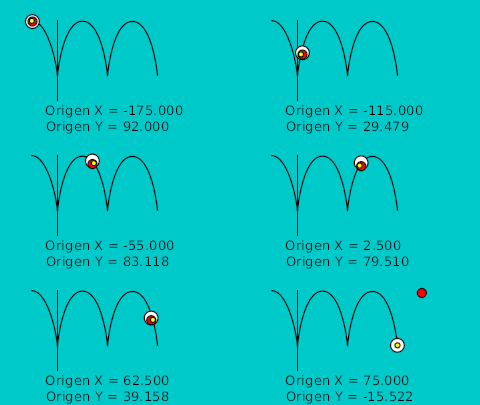
La regla para hacer el rebote manual es dibujar en un papel el rebote deseado. Después marcar la línea horizontal con intervalos regulares y hacerlos coincidir en la intersección de la curva en vertical. Véase la imagen:
Teniendo intervalos regulares en el eje horizontal (X) nos da intervalos irregulares en el eje vertival (Y). Esto se debe a la naturaleza de la curva.
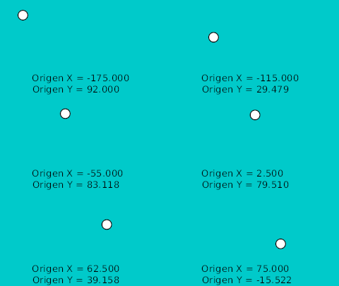
Once the points are located in a 2D grid then it can be drawn directly in Synfig doing use of the grid (F11). After drawing them we normalized the values to be completely symmetrical. That gives the following table:e
| Time | X position | Y position | Comments |
| 0f | -175.0 | 92.0 | Highest point |
| 4f | -165.0 | 92.0 | |
| 8f | -155.0 | 81.118 | |
| 12f | -145.0 | 63.678 | |
| 16f | -135.0 | 29.479 | |
| 20f | -125.0 | -15.522 | Lower point |
| 24f | -115.0 | 29.479 | |
| 28f | -105.0 | 63.782 | |
| ... | ... |
You can see that the X position is increasing in steps of 10.0 and the Y position reproduces a parabolic curve.
To proceed with more than one bounce just duplicate the waypoints (place the cursor at the right place right click over the waypoint and duplicate) reproducing symmetrical movements. You should need to edit the X values manually to decrease by 10.0 for each new waypoint.
This is the resulting graph for the manual approximation to the ball bounce.
The lower points are not peak points. To do that you need to insert more waypoints in intermediate places around the lower frame (20f). TRy it by your self with the attached file.
The resulting animation and file are those ones.
File: Media:manual.sifz
Ball Bounce using waypoints interpolations
The TCB interpolation mode allows modify the Tension, Continuity, Bias, and Temporal Tension values of the waypoint. So you can create easily smooth or peak aproximation to the value of the valuenode in the waypoint position.
This time I would use the same values for the highest and lower points of the table before. But I won't use more than one waypoint for each extreme position. The rest of the curve would be done using the TCB parameters.
The table of waypoints gives this result:
| Time | X position | Y position | Comments |
| 0f | -175.0 | 92.0 | Highest point |
| 20f | -125.0 | -15.522 | Lower point |
| 40f | -75.0 | 92.0 | Highest point |
| 60f | -25.0 | -15.522 | Lower point |
| ... | ... |
As you can see the number of points is reduced drastically.
In you only use a default TCB interpolation it would give you a poor result. Look at the graph:
But if you edit the TCB parameters this is the result you obtain:
The TCB parameters are the following:
| Time | X position | Y position | Comments | Tension | Continuity | Bias | Temporal Tension |
| 0f | -175.0 | 92.0 | Highest point | 0.0 | 0.0 | 0.0 | 0.0 |
| 20f | -125.0 | -15.522 | Lower point | 0.0 | -2.2 | 0.0 | 0.0 |
| 40f | -75.0 | 92.0 | Highest point | 0.0 | 0.0 | 0.0 | 0.0 |
| 60f | -25.0 | -15.522 | Lower point | 0.0 | -2.2 | 0.0 | 0.0 |
| 80f | 25.0 | 92.0 | Highest point | 0.0 | 0.0 | 0.0 | 0.0 |
| ... | ... | ... | ... | ... | ... | ... | ... |
That's the resulting animation:
And the sample file: Media:waypoint-2.sifz
Notice that the curve at 0f and at 80f are not properly formed. It is due to the fact that the TCB parameters needs to belong to an intermediate waypoint to have effect. If the waypoint is extreme (the end or the beginning of the animation for the parameter it cannot modify the curve. To solve that you should split the X and Y coordinates of the Origin and apply a Ease In/Out interpolation to those Y coordinate and leave the X coordinate with the current interpolation. So please consider only the bounces between the two black vertical lines.
Notice also that you can make the highest point more flat increasing the Temporal Tension parameter (a good value can be 0.5). This would produce a deformation to the X coordinate so you need to separate both coordinates to do that. Try it by your self editing the attached file. I have left the highest point to have the default values.
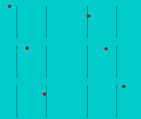
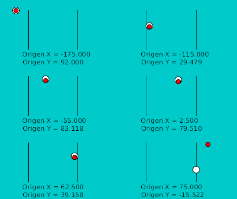
Here is a comparison of both bounces a the same time.
With this approximation you can easily modify the Y coordinate of the highest points. The interpolation would take care of the rest. With the manual interpolation you should calculate all the x/y coordinates od the resulting curve for a lower bounce. You can record the values into a calculus sheet and just multiply the Y value by a reduction factor. Anyway you have to enter all the value pairs one by one.
Ball Bounce following a path
To follow this section you should consider read the Follow a Bline tutorial. It makes use of that feature.
The use of a path to perform the bounce have some advantages.
- You can see the complete ball bounces in one shot.
- You can make the ball rotate along the path (this would allow make bounces of non rounded things).
- You can make bounces to vertical,horizontal or any kind of walls you like. Just draw the path.
It has some disadvantages:
- It is difficult to control the horizontal movement. It is due to the paramter that moves the object through the path is linked to the number of vertices vertices of the path. If the path have five vertices and it is an open Bline the parameter that defines the path has the following values when define each vertex: 0.0 for the first, 0.25 for the second, 0.5 for the third, 0.75 for the fourth and 1.0 for the fifth (and last) independent of the length of the Bline section between vertices.
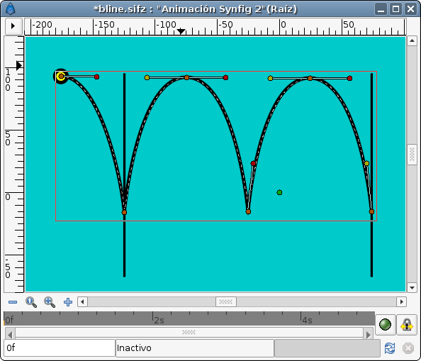
The first thing you have to do is define the path that the bouncing ball is going to describe. I've used the previous manual animation to draw this Bline:
(You can notice that there are some missing tangents. It is due that I've linked the parallel tangents of the peak points of the path. It is more easy to setup because you only have to control two tangents to control all the tangents at the same time.)
Once defined then create a circle or the ball you want to move and place it centred at the origin (0,0). I prefer that you encapsulate it and use the paste canvas origin parameter to make the animation. Once encapsulated select the bline you have created and the paste canvas of the encapsulated ball and select the Origin duck of the paste canvas. Then make right click over the bline (avoiding any duck) and select "Link to Bline". You can see my green ball in the figure.
Once linked you can drag it and it would be stick to the bline.
Now expand the Origin parameter of the paste canvas layer of the encapsulated ball and search for the Amount parameter. This parameter is the parameter you need to animate to move the ball over the Bline.
Considering the example, the bline has 6 vertices and 5 bline sections. If you are following the tutorial try to set that parameter to 0.0, 0.2, 0.4, 0.6, 0.8, 1.0 and you will see that the ball moves to each vertex. Now create the following waypoints:
| Time | Amount | Comments |
| 0f | 0.0 | Highest point |
| 20f | 0.2 | Lower point |
| 40f | 0.4 | Highest point |
| 60f | 0.6 | Lower point |
| 80f | 0.8 | Highest point |
| 100f | 1.0 | Lower point |
This coincides with the main waypoints of the last method we have seen. But look what's the result:
Its X movement graph looks ugly. It is not a straight line that means that the horizontal velocity is not constant. To solve that you have to insert more waypoints in the middle.
To do that I've uses the animation of the second method to try to match the position at regular intervals. This is the table I've needed.
| Time | Amount | Comments |
| 0f | 0.0 | Highest point |
| 20f | 0.2 | Lower point |
| 24f | 0.2626 | |
| 28f | 0.3085 | |
| 32f | 0.3463 | |
| 36f | 0.3741 | |
| 40f | 0.4 | Highest point |
| 44f | 0.4245 | |
| 48f | 0.4554 | |
| 52f | 0.4926 | |
| 56f | 0.5280 | |
| 60f | 0.6 | Lower point |
| 64f | 0.6629 | |
| 68f | 0.7075 | |
| 72f | 0.7445 | |
| 76f | 0.7783 | |
| 80f | 0.8 | Highest point |
| 84f | 0.8253 | |
| 88f | 0.8539 | |
| 92f | 0.8928 | |
| 96f | 0.9375 | |
| 100f | 1.0 | Lower point |
Now look to the graphs again and notice that the X travel is now a straight line.
This is the resulting animation and the sifz file.
The sample file: Media:bline.sifz
It is supposed that the small yellow ball should follow the red one all the time but you can see that is goes a little faster some times and a little slower other times. It is due to I need to use different times for the adjusting waypoints or add more of them.
Mathematical emulation
Anyone want to try? :)
